1) Linearity of QM
Example of linear theory: Maxwell’s Theory of electromagnetism
Assuming a plane wave propagating to the right being a solution to the set of equations, and another solution being a plane wave propagating out of page. Then, a third solution is their combination (superposition). This proves the linearity of the Maxwell equations and that the plane waves don’t affect each other.
Mathematically, , with being the current density, then linearity implies is also a solution, with .
Moreover, if and are solutions, then are also solutions.
It also includes some examples for linear and non-linear PDEs, so make sure to have a look.
Linear Equations
, is a linear operator, and is an unknown.
, ⇒
If , then is a solution.
Example & exercise: . In this exercise, the linear operator .
Now to verify the operator is linear, and .
Non-linear equations
Some may think Newton mechanics is simple, so it must be linear, but this is not the case. When a particle is moving under the influence of a potential , . While the LHS, the sum of derivatives is equal to the derivative of the sums, which is linear, the RHS might not be linear. If , , and that is not linear since .
How about QM? It is linear!
Schrödinger equation
represents the wavefunction which is dependent on time, is the Planck constant, and is the Hamiltonian, which is a linear operator.
An alternate form is , where . One advantage of this is that with one solution, we can construct much more solutions by scaling. With particles with spin, one or more wavefunctions may be needed to describe the mechanics.
2) Necessity of complex #s
Define the complex number ,
, and .
If lies on the unit circle (the circle centered at and has radius 1), can be written in the form
The norm of is Max Born discovered that the norm squared was proportional to the probabilities.
3) Loss in determinism
Einstein came up with the idea that light was made up of quanta of light, photons. A key difference between particles and waves are particles have zero size that carries energy, has a precise position and velocity. In the quantum mechanical world, it is thought of as an indivisible packet of energy or momentum that propagates.
For a photon, energy , where is the frequency of light. The frequency of light is related to by
A beam of light forming an angle to the x-axis can be represented as . When this light is passed through a polarizer that absorbs all light along the y-axis, the remaining is Now the energy of an electromagnetic field is proportional to the magnitude of the electric field squared. But the magnitude of the electric field is equal to .
Therefore, the fraction of energy through the polarizer is . Taking as an example, we check that the fraction of energy of a wave orthogonal to the polarizer is as all the energy is absorbed. In classical mechanics, if a photon gets absorbed, all identical photons should also be absorbed. If a photon goes through, all identical photons should also go through. But this is not the case. Some photons go through, and some are absorbed. Under identical experimental setting, we have different results. Then we’ve lost predictability when photons existed. A proposed explanation was, there is some property of photons that we haven’t discovered, and that determined whether a photon passes through a polarizer or not (hidden variable theory).
John Bell, with his famous Bell Inequality, proved that quantum mechanics cannot be made deterministic with hidden variables. Therefore, only probability can be used to determine whether a photon can pass through the polarizer.
Dirac invented the notation to represent a photon polarized in the x-direction: Likewise, a photon polarized in the y-direction can be represented as .
We have .
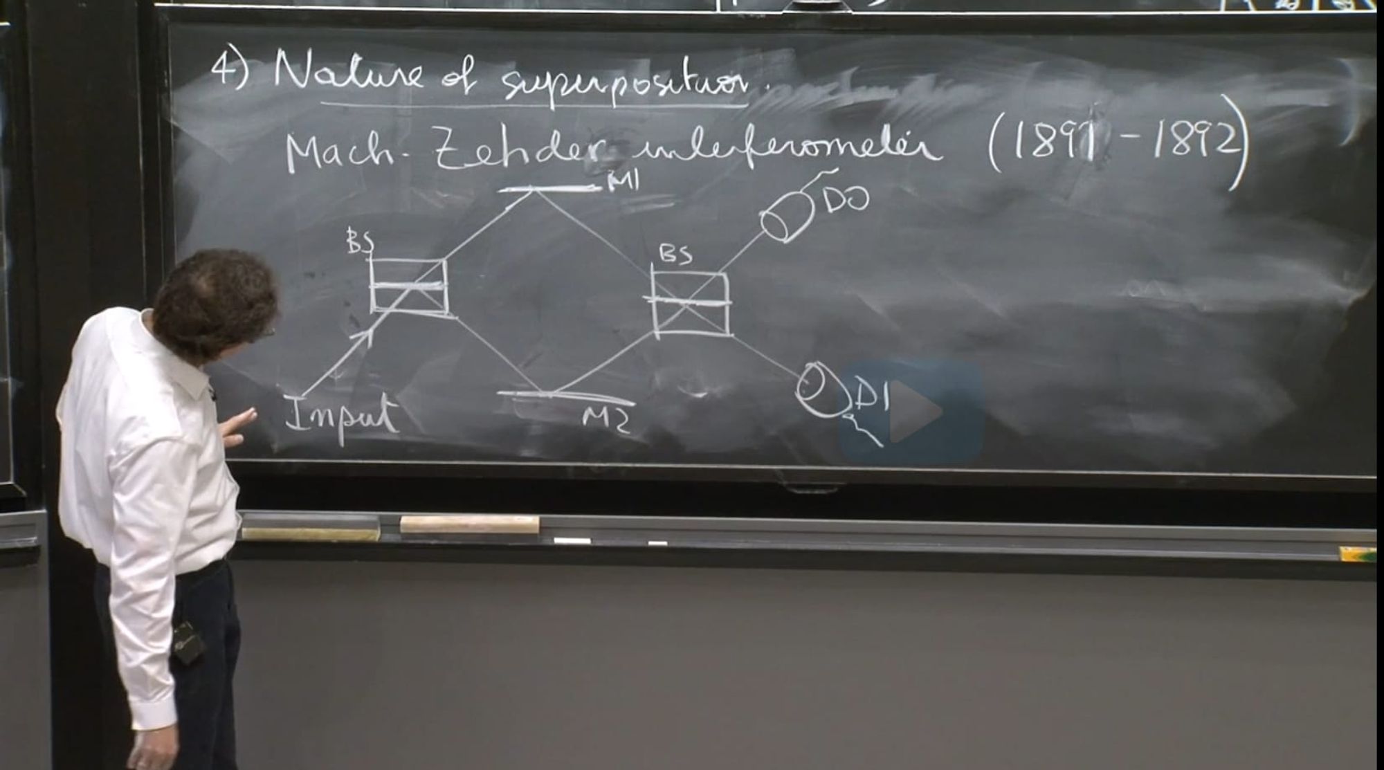
4) The nature of superposition
The nature of superposition can be illustrated with a Mach-Zehnder interferometer. We send in a beam of light, half of it gets transmitted, and half of it gets reflected. We take a beam splitter, breaking up a beam of light, and reflect it to recombine at a second beam splitter, and measure the intensity of the two beams of light.
Now we imagine the beam of light as a stream of protons travelling one by one. Some may think interference is the collision of photons. However, if interference was the collision of photons, a destructive interference would be equivalent to photons becoming packets of energy (with no light remaining), and a constructive interference is the addition of the electric field, making the amplitude 4 times greater since the amplitude is proportional to the field strength squared. However, this means 4 photons are created from 2 photons and this violates the law of conservation of energy. Therefore, when you get interference, it is interfering with itself.
A single photon is the superposition of a photon in the upper beam and a photon in the lower beam. A single photon is in both beams at the same time. When we measure a particle in the superposition , the probability of measuring state is , and the probability of measuring state is .
So in quantum mechanics, a measurement doesn’t yield an average results or an intermediate result. It leads to one or the other. This is also named the postulate of measurement.
Physical assumption: If we have a state, and superimpose it to itself, it is still physically equivalent compared to it before imposing. This means multiplying the physical state of your system has no relevance.
With representing physically equivalent, we can write:
It’s well known that polarized photons can be expressed with just two real parameters. With our property, we can reduce representing a polarized photon from with two real parameters to with only one complex parameter.
An elementary particle has intrinsic spin, and when we measure it along say the direction, the result can only be spin up or spin down with full magnitude. We represent these two results with:
5) Entanglement
In entanglement, we don’t need to have a strong interaction between particles to produce entanglement. Let’s consider particle 1, which can be of either state or state ; and particle 2, which can be of either state or state .
If particle 1 is doing , and particle 2 is doing , we can write this as . represents the tensor product. An important point to note is that the order of the product is non-exchangeable.
If particle 1 has state , and particle 2 has state , then their joint state is represented as
=
An example of an entangled state is . When we try to factor this state into separately, we find it is impossible. (This part is left to the reader as an exercise) So, we cannot describe this particular quantum state by telling what the first particle is doing and what the second particle is doing. They are dependent, and called an entangled state.
Let’s check out two spin particles, in the state . Say we measure the second particle, and it shows down spin. Then instantaneously, the first particle collapses to up spin. Somehow the two particles are connected to each other, but since the change is instantaneous, this violates special relativity, especially being the information exchange happening at faster than the speed of light.
Remember Mach-Zehnder interferometers?
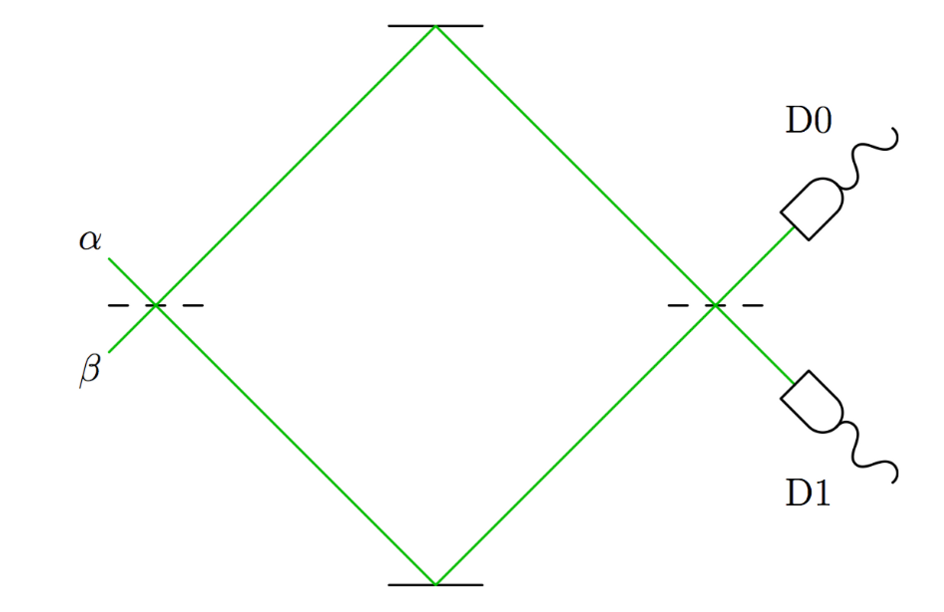
We can use two numbers to represent the probability amplitude for a photon to be in the upper beam and the lower beam. Mathematically, it can be written as .
The state represents the photons going to the upper beam, and likewise, means the photons going to the lower beam. Note that
for all and .
→
The beam splitter can be represented as the 2x2 matrix and act on a photon state. A balanced beam splitter makes half the beam go through, and the other half is reflected. Therefore, we can say . If you act on a normalized photon state, which satisfies , you should still get a normalized photon, since one photon will still come out as one photon. So to see if a beam splitter is constructable, we can check if its determinant is .
When inserting a phase shifter of phase in the lower leg of the apparatus, the new state can be obtained by multiplying quantum state by the matrix . Likewise, when inserting one in the upper leg of phase , the new state can be obtained by multiplying Finally, inserting a phase shifter of phase in the upper leg and a phase shifter of phase in the lower leg of the apparatus multiplies the quantum state by the matrix .
Elitzur-Vaidman bombs
We send the photon in through a tube within the bomb. If the photon is detected by the photon detector, the bomb explodes. On the other hand, of the bomb is defective, and the detector doesn’t work, the photon just passes through.
Puzzle: bombs decay over time, and sometimes the detectors don’t work anymore. Assume we can’t break down the bombs for inspection, and you want to test them. So the question is, is there a way to certify that the bomb is working without exploding it?
In classical physics, it’s impossible. If the bomb works, it’ll explode the moment you test it. However, we can insert this bomb in the Mach-Zehnder interferometer.
If we find photons coming out of D0, the test is inconclusive. If we find photons coming out of D1, we know that the bomb is working without detonating it!
For an in-detail explanation, feel free to visit this Wikipedia page.